

How To Change Binwidth In R
Visualise the distribution of a unmarried continuous variable by dividing the x axis into bins and counting the number of observations in each bin. Histograms (geom_histogram()) display the counts with confined; frequency polygons (geom_freqpoly()) display the counts with lines. Frequency polygons are more suitable when y'all want to compare the distribution beyond the levels of a categorical variable.
Usage
geom_freqpoly ( mapping = Cypher, information = NULL, stat = "bin", position = "identity", ..., na.rm = Imitation, show.fable = NA, inherit.aes = TRUE ) geom_histogram ( mapping = NULL, data = NULL, stat = "bin", position = "stack", ..., binwidth = Nil, bins = Nil, na.rm = Fake, orientation = NA, show.legend = NA, inherit.aes = TRUE ) stat_bin ( mapping = Nada, data = Zilch, geom = "bar", position = "stack", ..., binwidth = Naught, bins = Zero, center = NULL, purlieus = NULL, breaks = NULL, closed = c ( "right", "left" ), pad = FALSE, na.rm = FALSE, orientation = NA, show.legend = NA, inherit.aes = Truthful ) Arguments
- mapping
-
Ready of artful mappings created by
aes(). If specified andinherit.aes = True(the default), information technology is combined with the default mapping at the height level of the plot. You lot must supplymappingif there is no plot mapping. - data
-
The data to be displayed in this layer. There are iii options:
If
Zippo, the default, the data is inherited from the plot data as specified in the call toggplot().A
data.frame, or other object, will override the plot data. All objects will exist fortified to produce a information frame. Seefortify()for which variables will be created.A
functionwill exist called with a unmarried argument, the plot data. The return value must be ainformation.frame, and will be used as the layer data. Aroletin can exist created from aformula(eastward.thousand.~ head(.x, x)). - position
-
Position adjustment, either every bit a string naming the aligning (e.g.
"jitter"to utiliseposition_jitter), or the result of a call to a position adjustment function. Apply the latter if you need to change the settings of the adjustment. - ...
-
Other arguments passed on to
layer(). These are often aesthetics, used to set an aesthetic to a stock-still value, similarcolor = "red"orsize = 3. They may as well be parameters to the paired geom/stat. - na.rm
-
If
FALSE, the default, missing values are removed with a warning. IfTRUE, missing values are silently removed. - bear witness.legend
-
logical. Should this layer be included in the legends?
NA, the default, includes if whatever aesthetics are mapped.FALSEnever includes, andTRUEalways includes. It tin can as well be a named logical vector to finely select the aesthetics to display. - inherit.aes
-
If
FALSE, overrides the default aesthetics, rather than combining with them. This is most useful for helper functions that define both data and aesthetics and shouldn't inherit behaviour from the default plot specification, e.m.borders(). - binwidth
-
The width of the bins. Can be specified every bit a numeric value or equally a function that calculates width from unscaled x. Hither, "unscaled x" refers to the original ten values in the data, earlier application of whatever scale transformation. When specifying a role along with a grouping structure, the function will be chosen once per group. The default is to use the number of bins in
bins, covering the range of the data. You lot should always override this value, exploring multiple widths to find the best to illustrate the stories in your data.The bin width of a date variable is the number of days in each time; the bin width of a fourth dimension variable is the number of seconds.
- bins
-
Number of bins. Overridden by
binwidth. Defaults to 30. - orientation
-
The orientation of the layer. The default (
NA) automatically determines the orientation from the aesthetic mapping. In the rare consequence that this fails information technology can be given explicitly past settingorientationto either"x"or"y". See the Orientation section for more detail. - geom, stat
-
Utilize to override the default connection between
geom_histogram()/geom_freqpoly()andstat_bin(). - center, boundary
-
bin position specifiers. Only one,
centerorboundary, may exist specified for a single plot.centerspecifies the center of ane of the bins.purlieusspecifies the boundary between two bins. Notation that if either is above or below the range of the data, things will exist shifted by the appropriate integer multiple ofbinwidth. For case, to middle on integers usebinwidth = iandcentre = 0, even if0is outside the range of the data. Alternatively, this same alignment can be specified withbinwidth = 1andboundary = 0.5, even if0.fiveis outside the range of the data. - breaks
-
Alternatively, you lot can supply a numeric vector giving the bin boundaries. Overrides
binwidth,bins,heart, andpurlieus. - closed
-
1 of
"right"or"left"indicating whether correct or left edges of bins are included in the bin. - pad
-
If
TRUE, adds empty bins at either end of x. This ensures frequency polygons touch 0. Defaults toFALSE.
Details
stat_bin() is suitable just for continuous x information. If your ten information is discrete, yous probably want to use stat_count().
Past default, the underlying computation (stat_bin()) uses 30 bins; this is not a expert default, merely the idea is to get you experimenting with different number of bins. You can also experiment modifying the binwidth with center or purlieus arguments. binwidth overrides bins so yous should exercise one modify at a time. You may demand to look at a few options to uncover the full story backside your data.
In improver to geom_histogram(), you tin create a histogram plot by using scale_x_binned() with geom_bar(). This method by default plots tick marks in between each bar.
Orientation
This geom treats each axis differently and, thus, tin can thus have two orientations. Ofttimes the orientation is easy to deduce from a combination of the given mappings and the types of positional scales in use. Thus, ggplot2 will by default try to guess which orientation the layer should have. Under rare circumstances, the orientation is ambiguous and guessing may fail. In that case the orientation tin can exist specified straight using the orientation parameter, which can be either "ten" or "y". The value gives the axis that the geom should run along, "x" beingness the default orientation you would expect for the geom.
Aesthetics
geom_histogram() uses the same aesthetics as geom_bar(); geom_freqpoly() uses the same aesthetics as geom_line().
Computed variables
-
count -
number of points in bin
-
density -
density of points in bin, scaled to integrate to 1
-
ncount -
count, scaled to maximum of 1
-
ndensity -
density, scaled to maximum of 1
-
width -
widths of bins
Dropped variables
-
weight -
Subsequently binning, weights of individual information points (if supplied) are no longer available.
See as well
stat_count(), which counts the number of cases at each ten position, without binning. It is suitable for both discrete and continuous x data, whereas stat_bin() is suitable simply for continuous 10 data.
Examples
ggplot ( diamonds, aes ( carat ) ) + geom_histogram ( ) #> `stat_bin()` using `bins = 30`. Pick better value with `binwidth`. 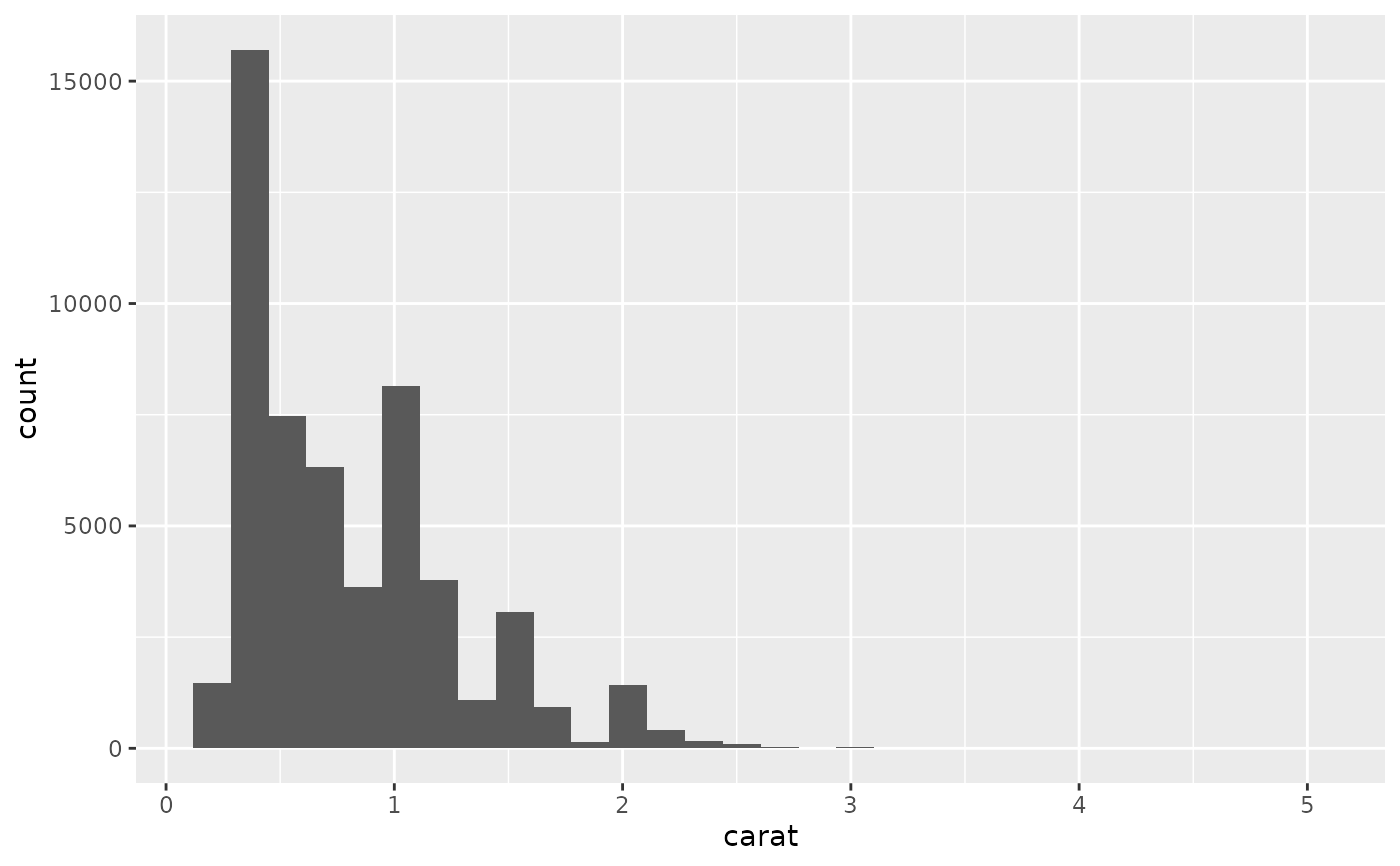 ggplot ( diamonds, aes ( carat ) ) + geom_histogram (binwidth = 0.01 )
 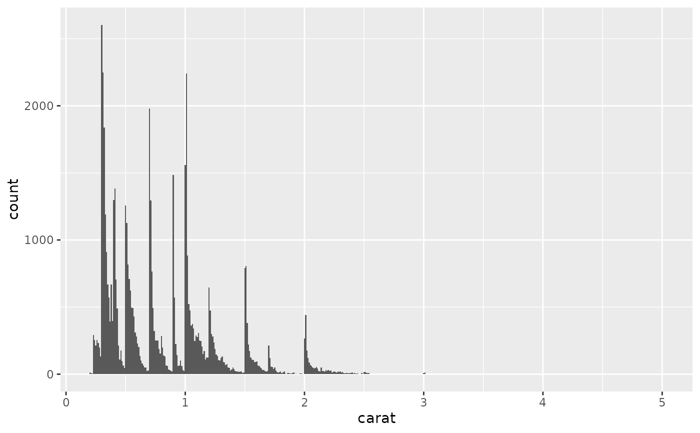 ggplot ( diamonds, aes ( carat ) ) + geom_histogram (bins = 200 )
 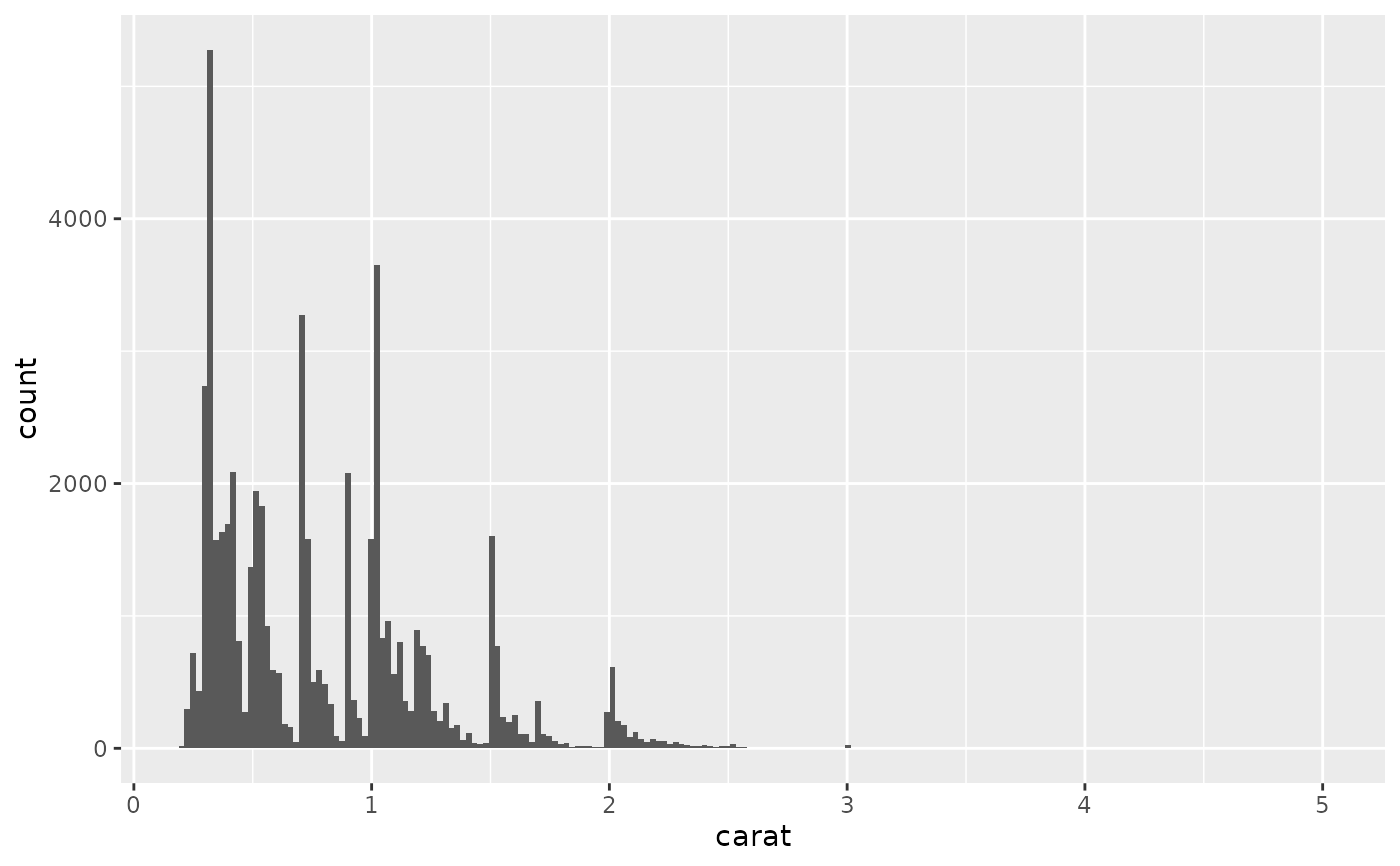 # Map values to y to flip the orientation ggplot ( diamonds, aes (y = carat ) ) + geom_histogram ( ) #> `stat_bin()` using `bins = thirty`. Pick better value with `binwidth`.
 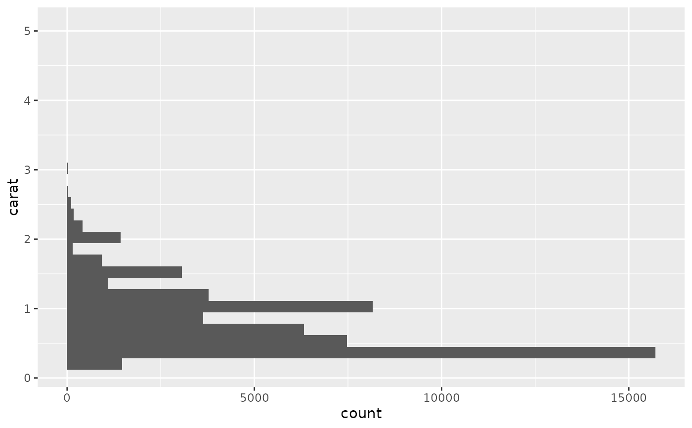 # For histograms with tick marks betwixt each bin, use `geom_bar()` with # `scale_x_binned()`. ggplot ( diamonds, aes ( carat ) ) + geom_bar ( ) + scale_x_binned ( )
 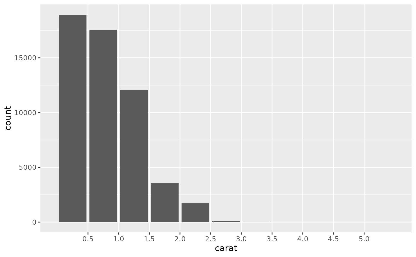 # Rather than stacking histograms, it's easier to compare frequency # polygons ggplot ( diamonds, aes ( cost, fill up = cutting ) ) + geom_histogram (binwidth = 500 )
 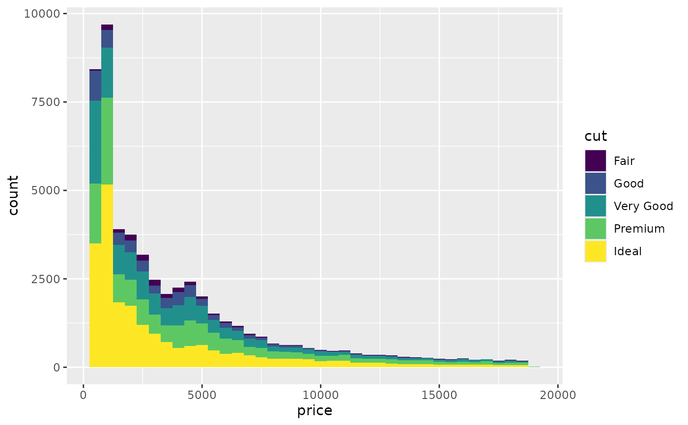 ggplot ( diamonds, aes ( cost, color = cutting ) ) + geom_freqpoly (binwidth = 500 )
 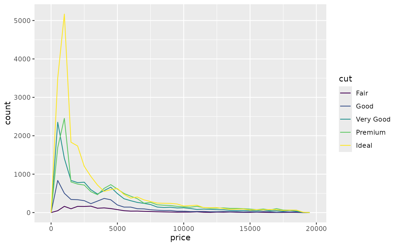 # To make it easier to compare distributions with very different counts, # put density on the y centrality instead of the default count ggplot ( diamonds, aes ( price, after_stat ( density ), colour = cut ) ) + geom_freqpoly (binwidth = 500 )
 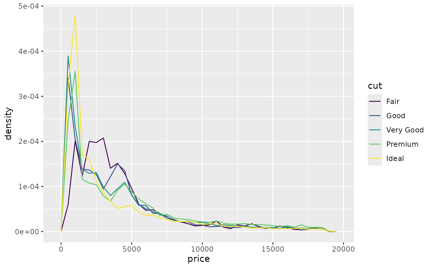 if ( require ( "ggplot2movies" ) ) { # Often we don't want the height of the bar to represent the # count of observations, but the sum of some other variable. # For example, the following plot shows the number of movies # in each rating. chiliad <- ggplot ( movies, aes ( rating ) ) m + geom_histogram (binwidth = 0.1 ) # If, however, we want to run across the number of votes cast in each # category, we demand to weight by the votes variable yard + geom_histogram ( aes (weight = votes ), binwidth = 0.1 ) + ylab ( "votes" ) # For transformed scales, binwidth applies to the transformed data. # The bins accept constant width on the transformed calibration. chiliad + geom_histogram ( ) + scale_x_log10 ( ) thou + geom_histogram (binwidth = 0.05 ) + scale_x_log10 ( ) # For transformed coordinate systems, the binwidth applies to the # raw information. The bins have constant width on the original scale. # Using log scales does not work here, because the first # bar is anchored at zero, and so when transformed becomes negative # infinity. This is not a problem when transforming the scales, because # no observations accept 0 ratings. m + geom_histogram (boundary = 0 ) + coord_trans (ten = "log10" ) # Apply boundary = 0, to make sure nosotros don't have sqrt of negative values m + geom_histogram (boundary = 0 ) + coord_trans (10 = "sqrt" ) # You tin too transform the y axis. Remember that the base of the bars # has value 0, then log transformations are not advisable chiliad <- ggplot ( movies, aes (ten = rating ) ) m + geom_histogram (binwidth = 0.5 ) + scale_y_sqrt ( ) }
 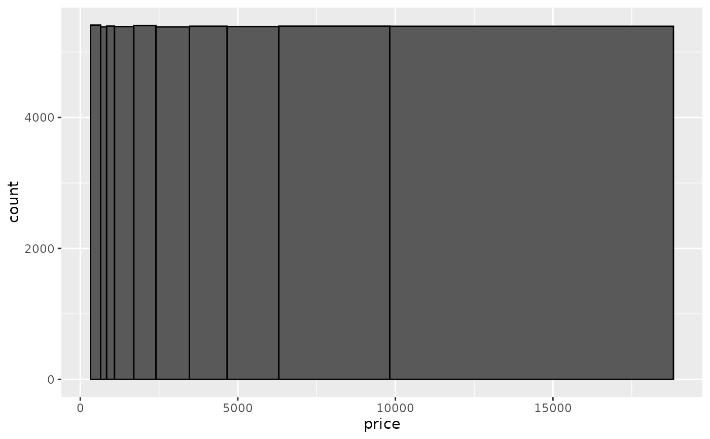 # You tin specify a function for calculating binwidth, which is # particularly useful when faceting along variables with # different ranges because the function volition be called once per facet ggplot ( economics_long, aes ( value ) ) + facet_wrap ( ~ variable, scales = 'free_x' ) + geom_histogram (binwidth = function ( x ) 2 * IQR ( ten ) / ( length ( ten ) ^ ( one / 3 ) ) )
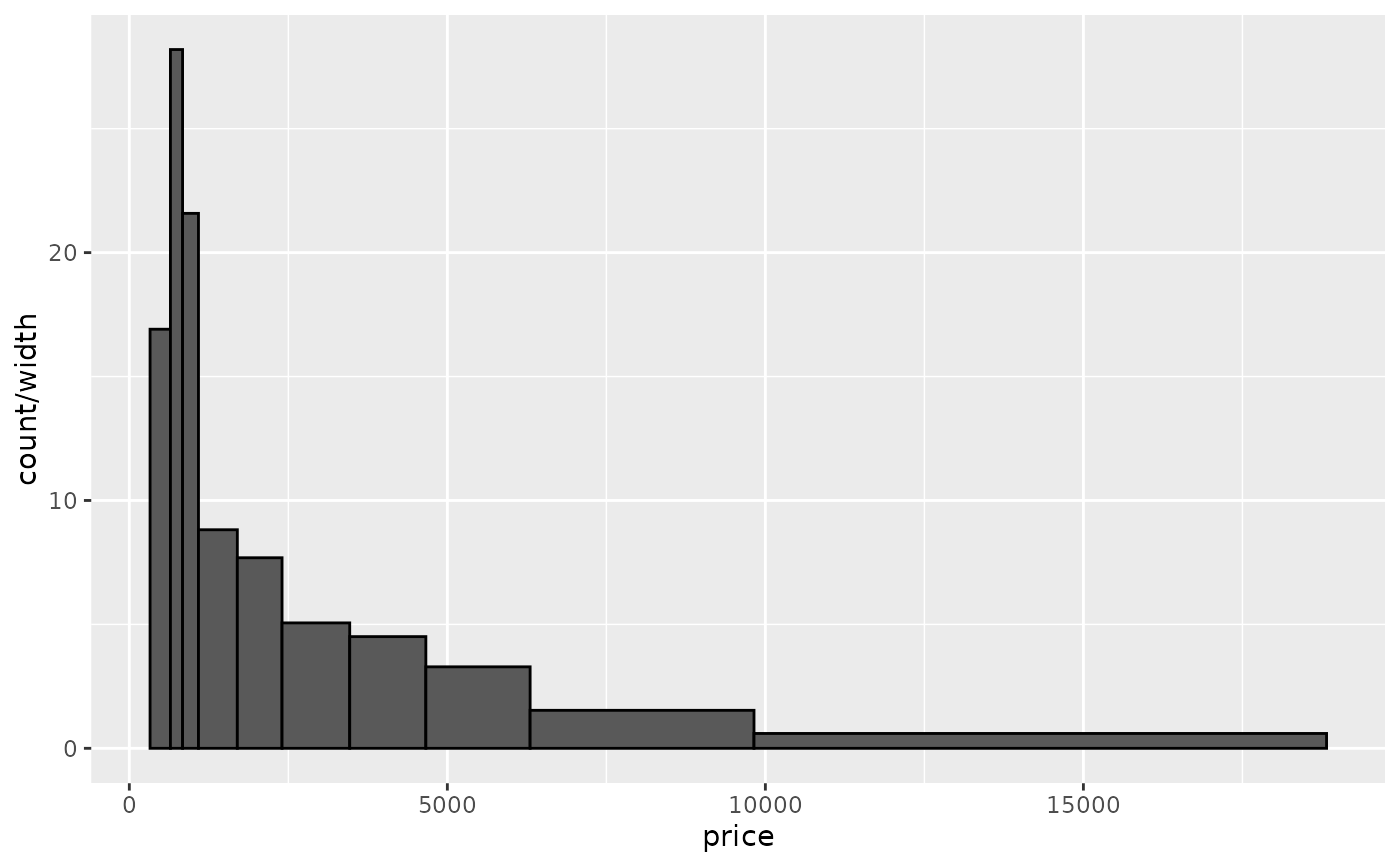
Source: https://ggplot2.tidyverse.org/reference/geom_histogram.html
0 Response to "How To Change Binwidth In R"
Post a Comment